artyfarty focuses on providing easy access to a few ‘nice’ ggplot theme, it also includes a number of predefined palettes and watermark convenience functions.

artyfarty is a work in progress. For now you can install the development version using devtools.

devtools::install_github('datarootsio/artyfarty')

Available themes

dataroots

ggplot(diamonds) +
  geom_bar(aes(cut, fill=cut)) +
  theme_dataroots() +
  ggtitle("Sparkly stones") +
  scale_fill_manual(values = pal("dataroots"))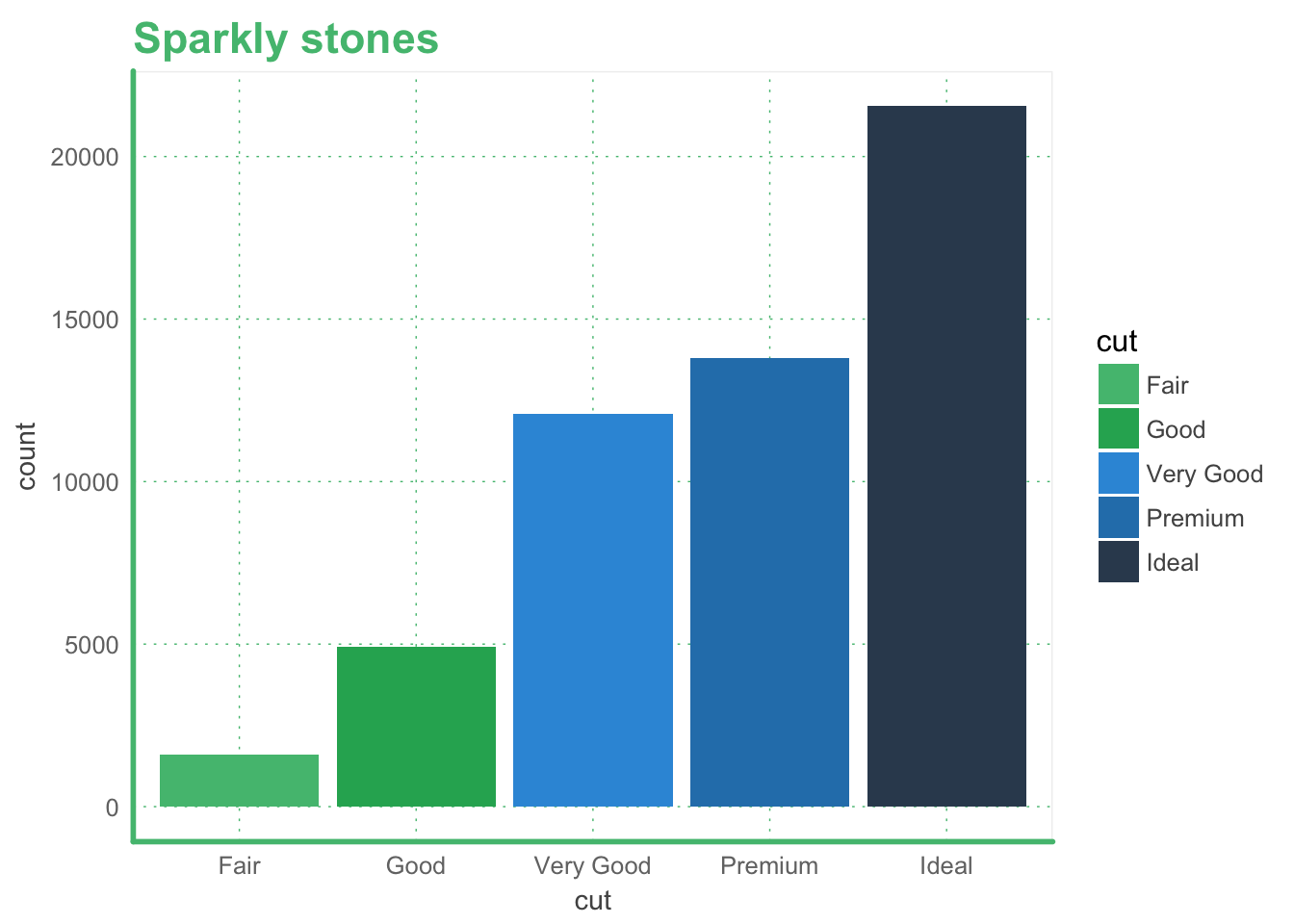

ggplot(mtcars) +
  geom_point(aes(x=wt, y=qsec, color=as.factor(cyl))) +
  theme_dataroots() +
  ggtitle("Vroom") +
  scale_color_manual(values = pal("dataroots"))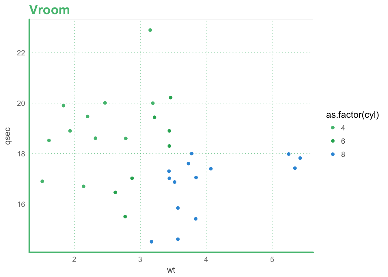

farty

ggplot(diamonds) +
  geom_bar(aes(cut, fill=cut)) +
  theme_farty() +
  ggtitle("Sparkly stones") +
  scale_fill_manual(values = pal("flat"))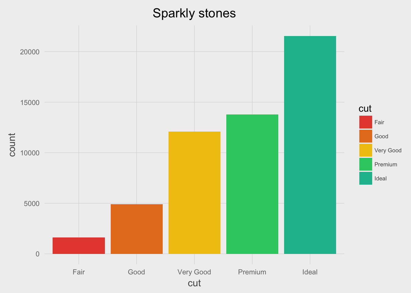

ggplot(mtcars) +
  geom_point(aes(x=wt, y=qsec, color=as.factor(cyl))) +
  theme_farty() +
  ggtitle("Vroom") +
  scale_color_manual(values = pal("flat"))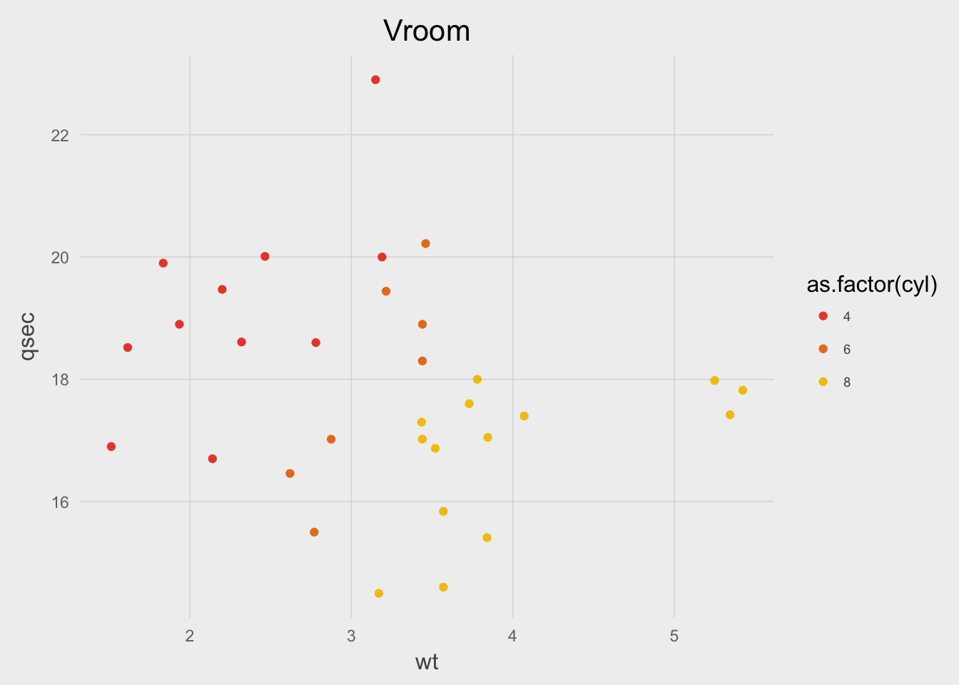

scientific

ggplot(diamonds) +
  geom_bar(aes(cut, fill=cut)) +
  theme_scientific() +
  ggtitle("Sparkly stones") +
  scale_fill_manual(values = pal("five38"))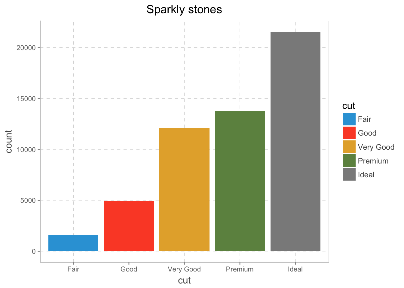

ggplot(mtcars) +
  geom_point(aes(x=wt, y=qsec, color=as.factor(cyl))) +
  theme_scientific() +
  ggtitle("Vroom") +
  scale_color_manual(values = pal("five38"))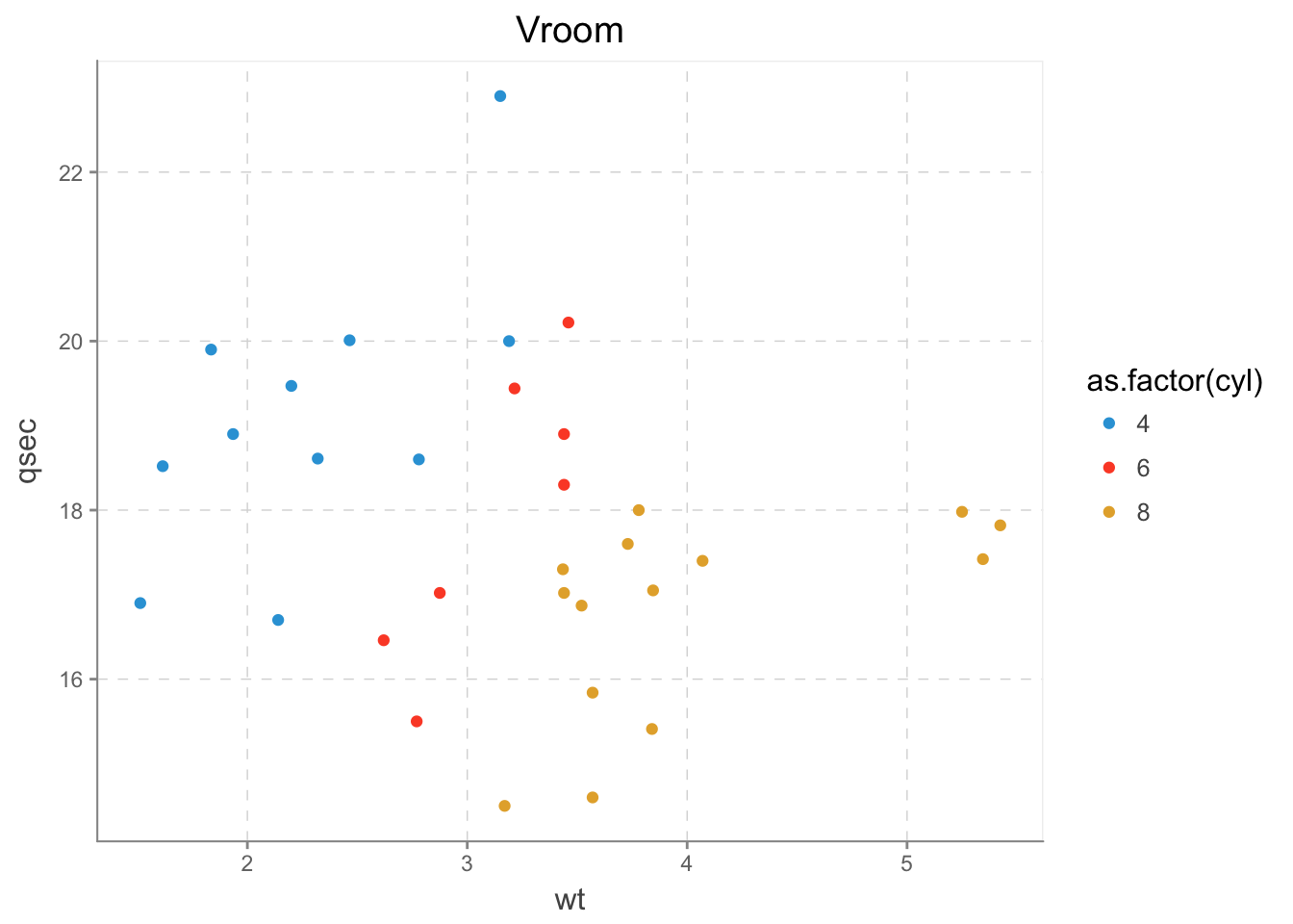

monokai

ggplot(diamonds) +
  geom_bar(aes(cut, fill=cut)) +
  theme_monokai() +
  ggtitle("Sparkly stones") +
  scale_fill_manual(values = pal("monokai"))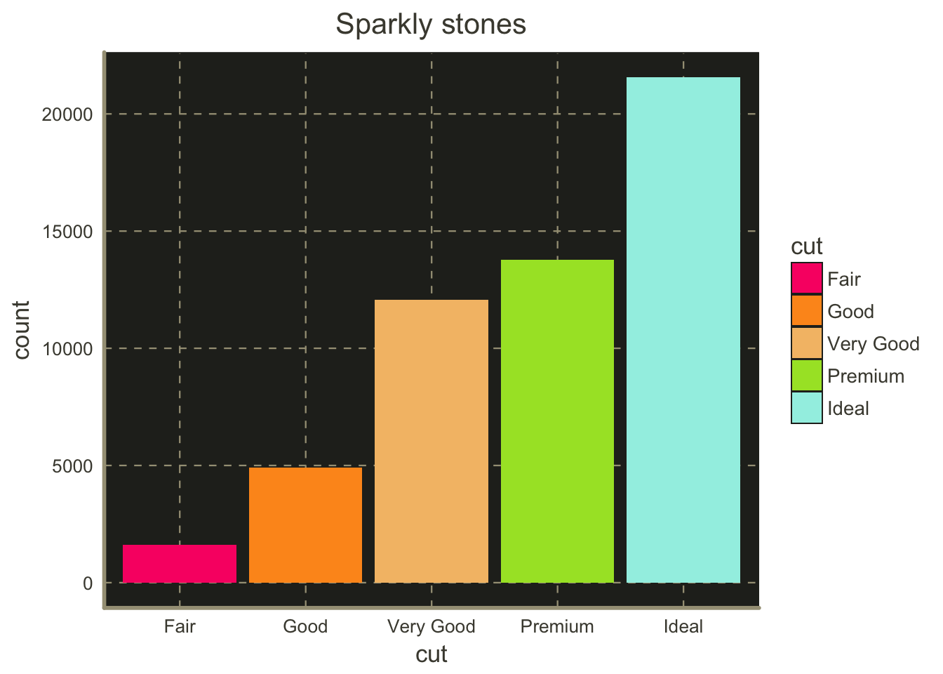

ggplot(mtcars) +
  geom_point(aes(x=wt, y=qsec, color=as.factor(cyl))) +
  theme_monokai() +
  ggtitle("Vroom") +
  scale_color_manual(values = pal("monokai"))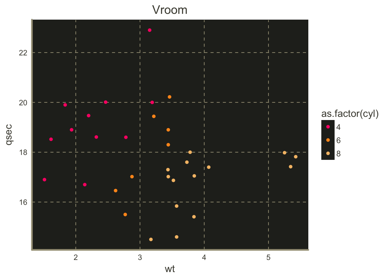

monokai_full

ggplot(diamonds) +
  geom_bar(aes(cut, fill=cut)) +
  theme_monokai_full() +
  ggtitle("Sparkly stones") +
  scale_fill_manual(values = pal("monokai"))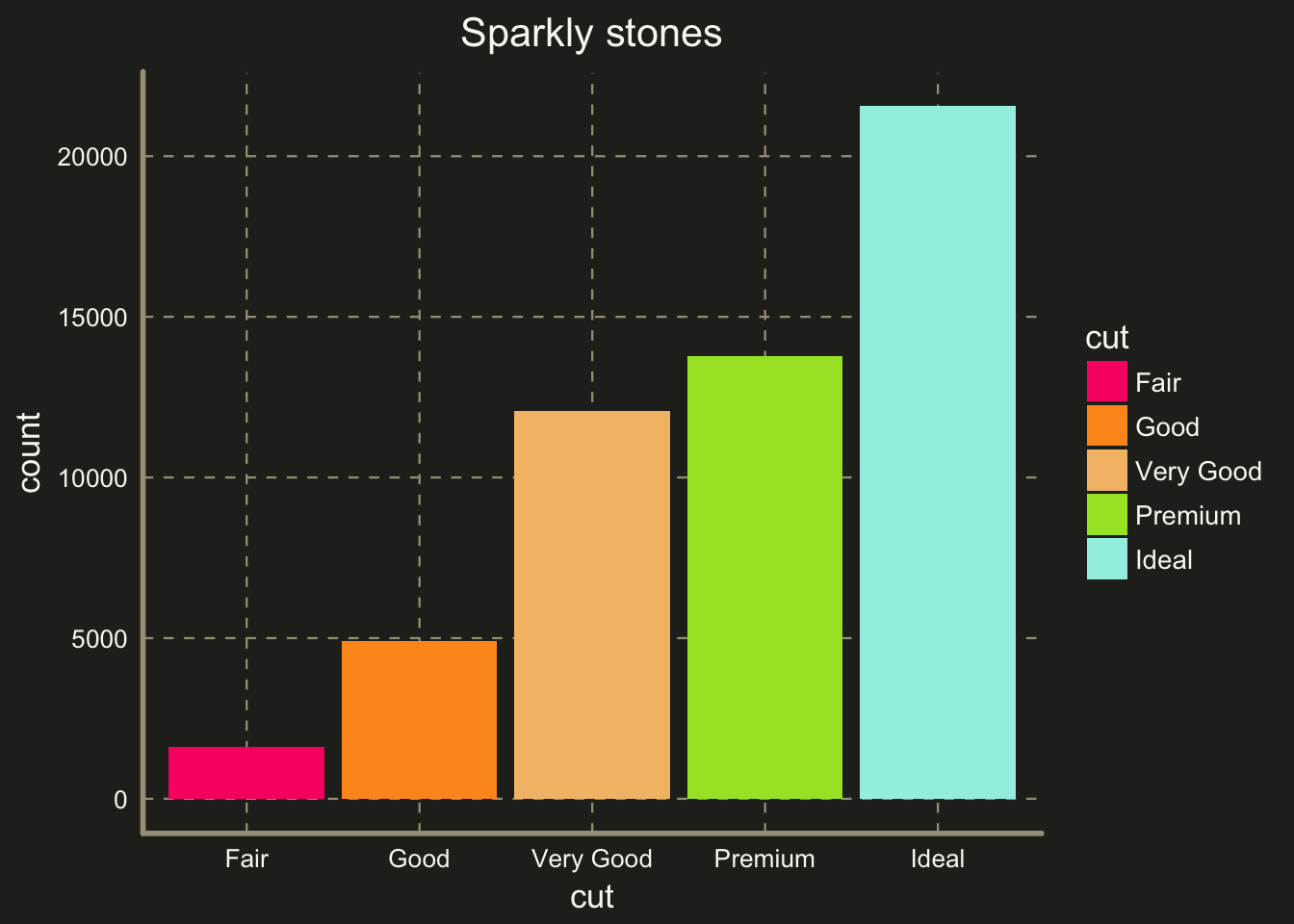

ggplot(mtcars) +
  geom_point(aes(x=wt, y=qsec, color=as.factor(cyl))) +
  theme_monokai_full() +
  ggtitle("Vroom") +
  scale_color_manual(values = pal("monokai"))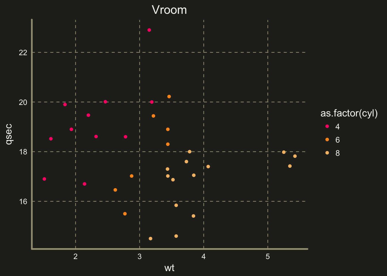

flat

ggplot(diamonds) +
  geom_bar(aes(cut, fill=cut)) +
  theme_flat() +
  ggtitle("Sparkly stones") +
  scale_fill_manual(values = pal("flat"))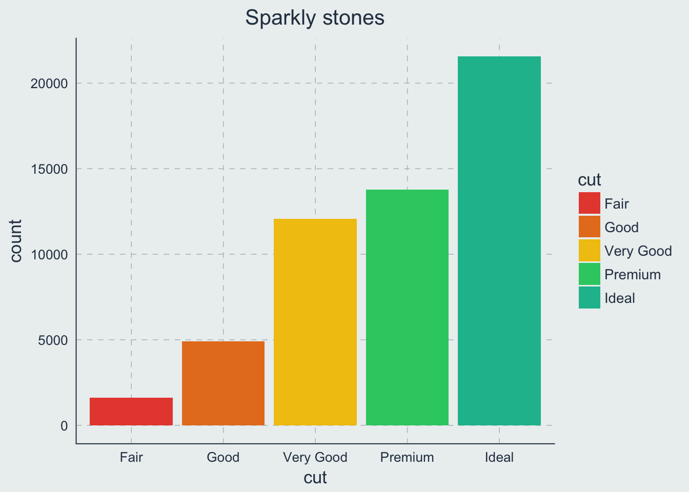

ggplot(mtcars) +
  geom_point(aes(x=wt, y=qsec, color=as.factor(cyl))) +
  theme_flat() +
  ggtitle("Vroom") +
  scale_color_manual(values = pal("flat"))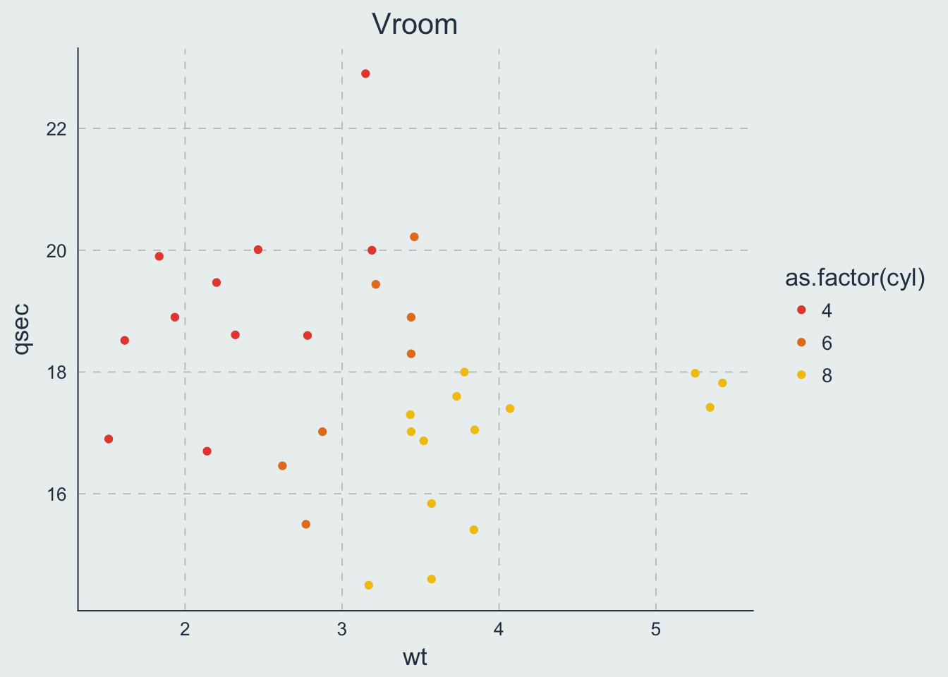

five38

ggplot(diamonds) +
  geom_bar(aes(cut, fill=cut)) +
  theme_five38() +
  ggtitle("Sparkly stones") +
  scale_fill_manual(values = pal("five38"))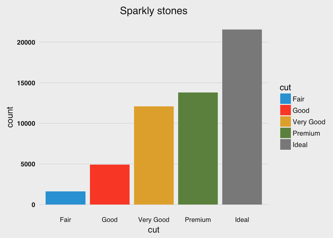

ggplot(diamonds) +
  geom_bar(aes(cut, fill=cut)) +
  theme_five38(grid_lines = "horizontal") +
  ggtitle("Sparkly stones") +
  scale_fill_manual(values = pal("five38")) +
  coord_flip()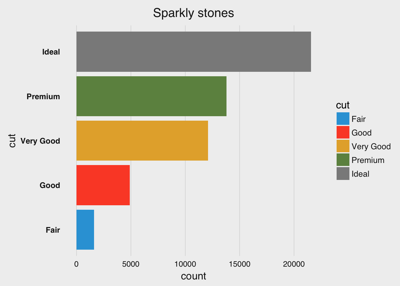

ggplot(mtcars) +
  geom_point(aes(x=wt, y=qsec, color=as.factor(cyl))) +
  theme_five38() +
  ggtitle("Vroom") +
  scale_color_manual(values = pal("five38"))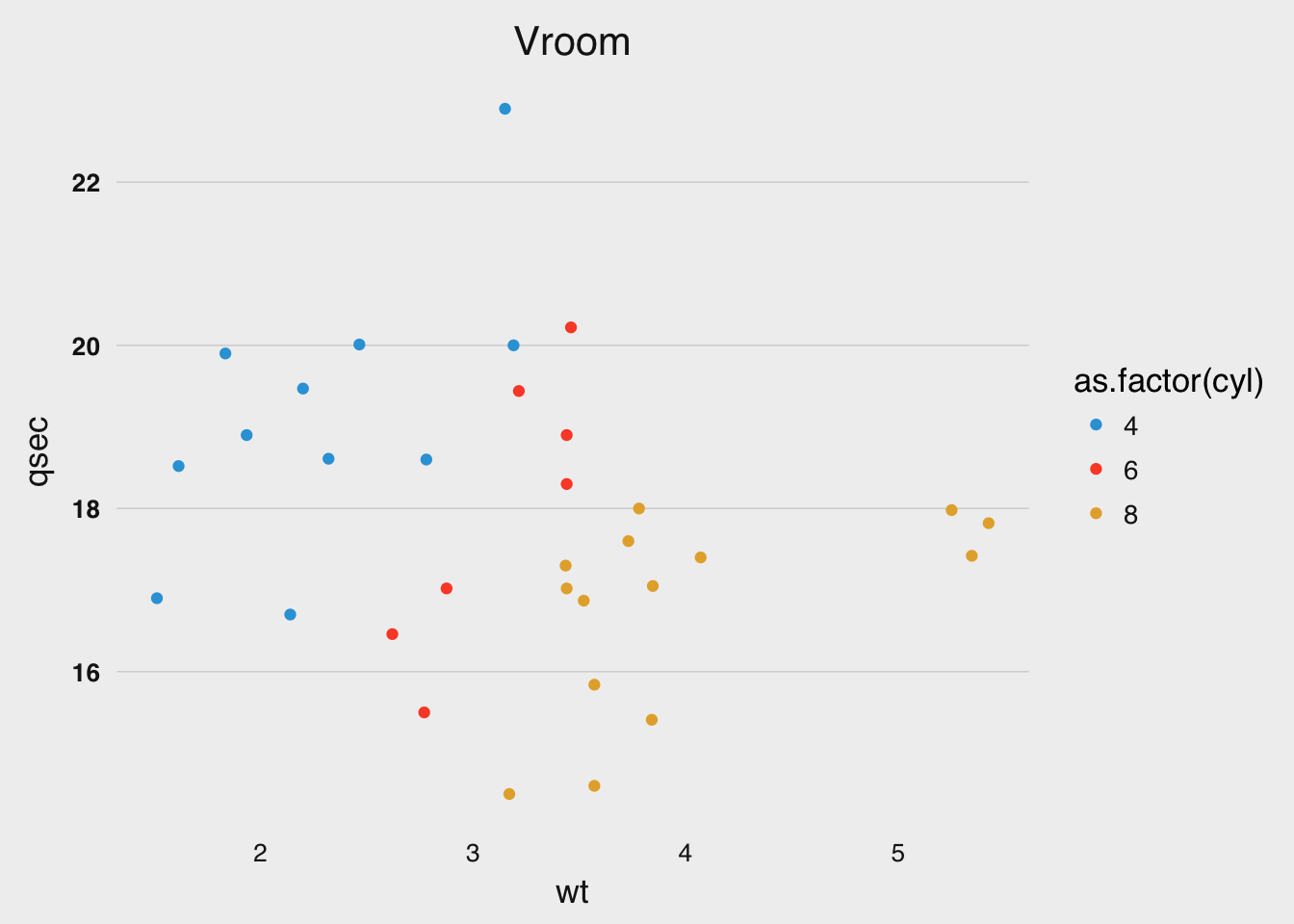

retro

ggplot(diamonds) +
  geom_bar(aes(cut, fill=cut)) +
  theme_retro() +
  ggtitle("Sparkly stones") +
  scale_fill_manual(values = pal("retro"))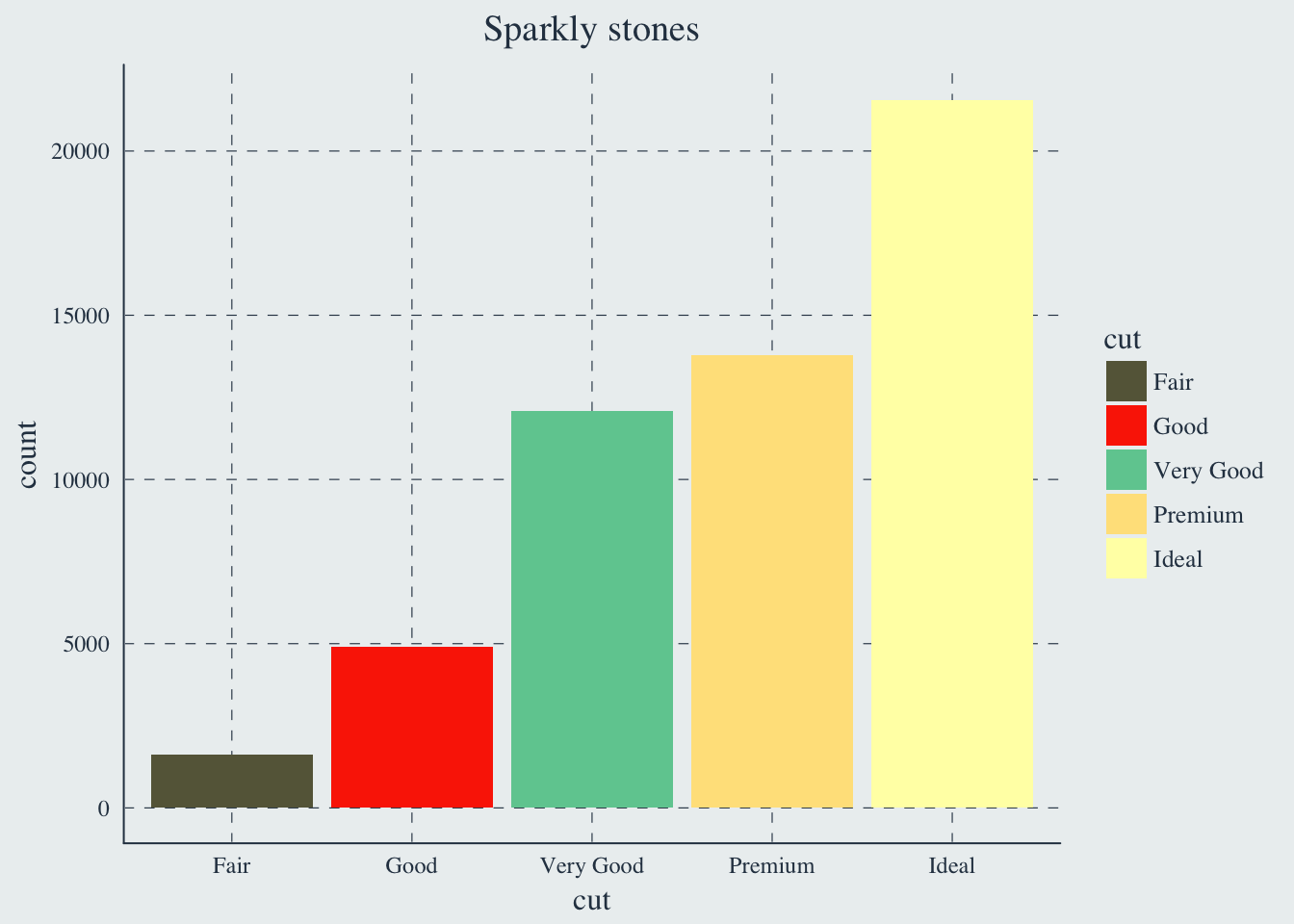

ggplot(mtcars) +
  geom_point(aes(x=wt, y=qsec, color=as.factor(cyl))) +
  theme_retro() +
  ggtitle("Vroom") +
  scale_color_manual(values = pal("retro"))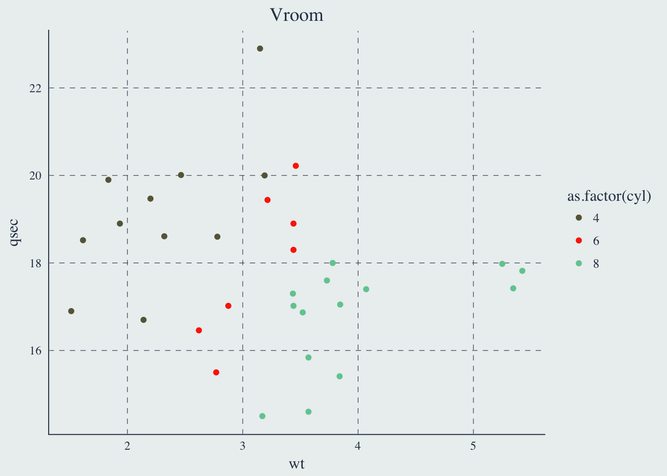

ft

ggplot(diamonds) +
  geom_bar(aes(cut, fill=cut)) +
  theme_ft() +
  ggtitle("Sparkly stones") +
  scale_fill_manual(values = pal("ft"))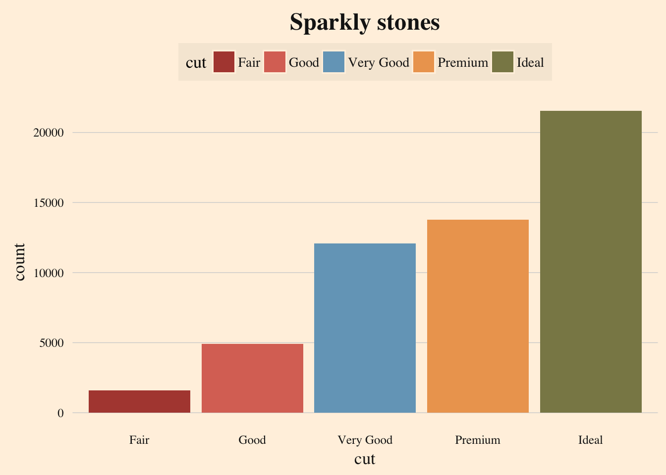

ggplot(diamonds) +
  geom_bar(aes(cut, fill=cut)) +
  theme_ft(grid_lines = "horizontal") +
  ggtitle("Sparkly stones") +
  scale_fill_manual(values = pal("ft")) +
  coord_flip()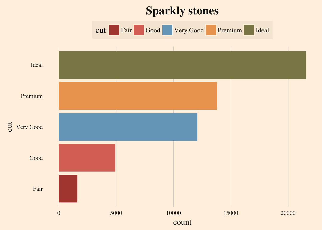

ggplot(mtcars) +
  geom_point(aes(x=wt, y=qsec, color=as.factor(cyl))) +
  theme_ft() +
  ggtitle("Vroom") +
  scale_color_manual(values = pal("ft"))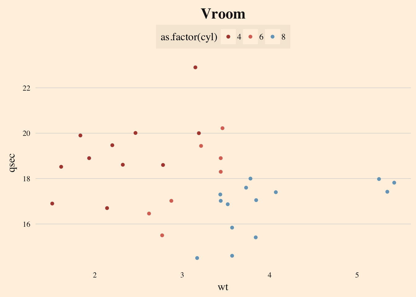

bain

ggplot(diamonds) +
  geom_bar(aes(cut, fill=cut)) +
  theme_bain() +
  ggtitle("Sparkly stones") +
  scale_fill_manual(values = pal("bain"))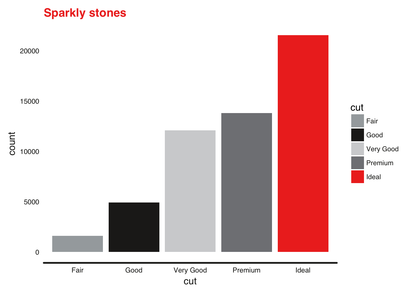

ggplot(diamonds) +
  geom_bar(aes(cut, fill=cut)) +
  theme_bain(grid_lines = "horizontal") +
  ggtitle("Sparkly stones") +
  scale_fill_manual(values = pal("bain")) +
  coord_flip()

ggplot(mtcars) +
  geom_point(aes(x=wt, y=qsec, color=as.factor(cyl))) +
  theme_bain() +
  ggtitle("Vroom") +
  scale_color_manual(values = pal("bain"))

economist

ggplot(diamonds) +
  geom_bar(aes(cut, fill=cut)) +
  theme_economist() +
  ggtitle("Sparkly stones") +
  scale_fill_manual(values = pal("economist"))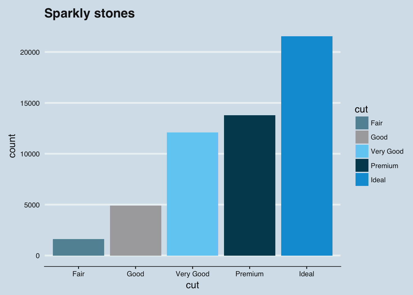

ggplot(diamonds) +
  geom_bar(aes(cut, fill=cut)) +
  theme_economist(grid_lines = "horizontal") +
  ggtitle("Sparkly stones") +
  scale_fill_manual(values = pal("economist")) +
  coord_flip()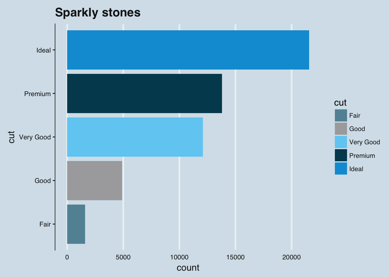

ggplot(mtcars) +
  geom_point(aes(x=wt, y=qsec, color=as.factor(cyl))) +
  theme_economist() +
  ggtitle("Vroom") +
  scale_color_manual(values = pal("economist"))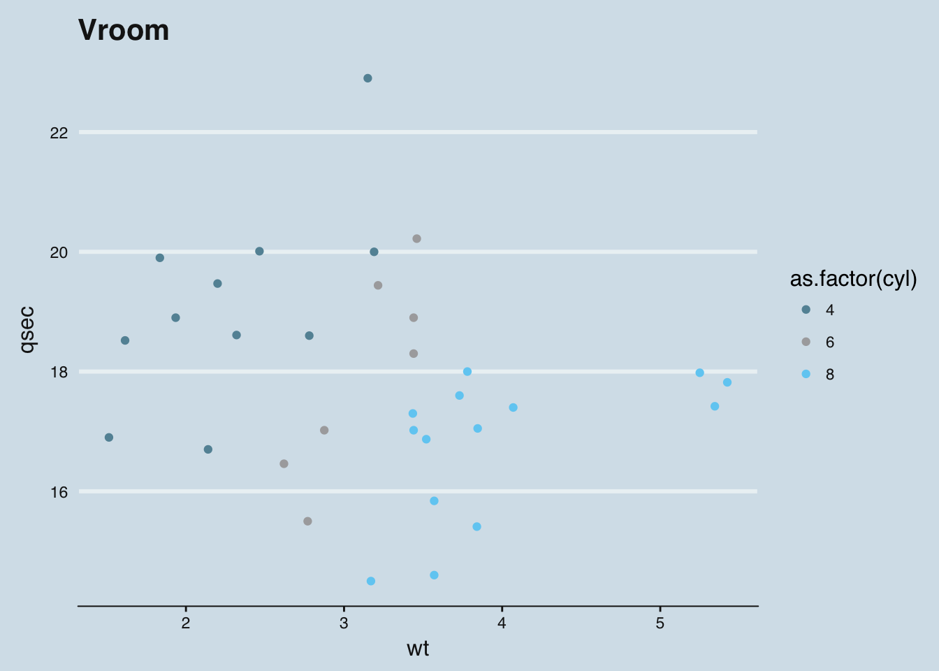

empty

ggplot(diamonds) +
  geom_bar(aes(cut, fill=cut)) +
  theme_empty() +
  ggtitle("Sparkly stones") +
  scale_fill_manual(values = pal("flat"))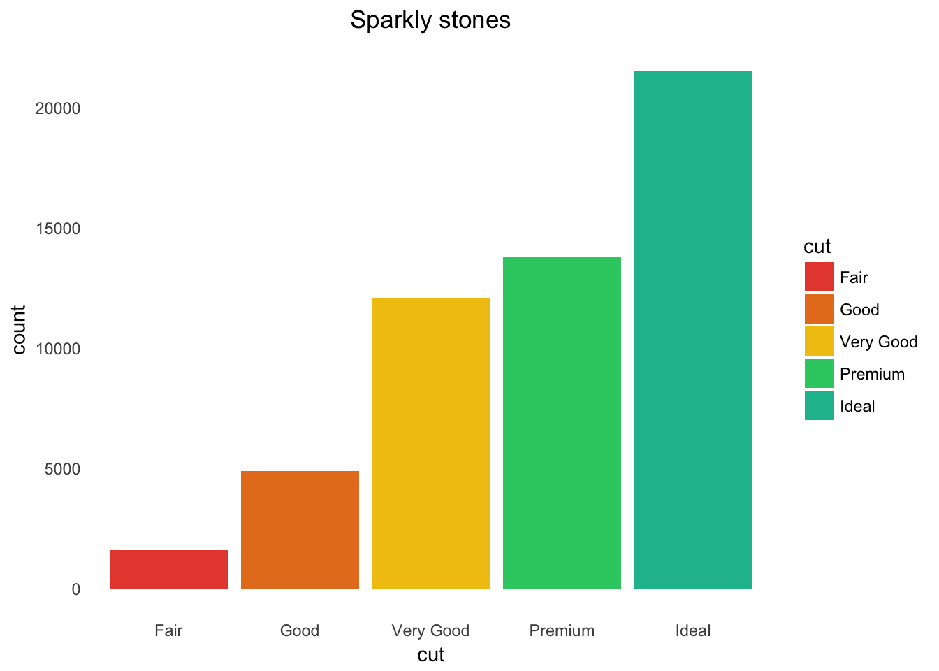

ggplot(mtcars) +
  geom_point(aes(x=wt, y=qsec, color=as.factor(cyl))) +
  theme_empty() +
  ggtitle("Vroom") +
  scale_color_manual(values = pal("flat"))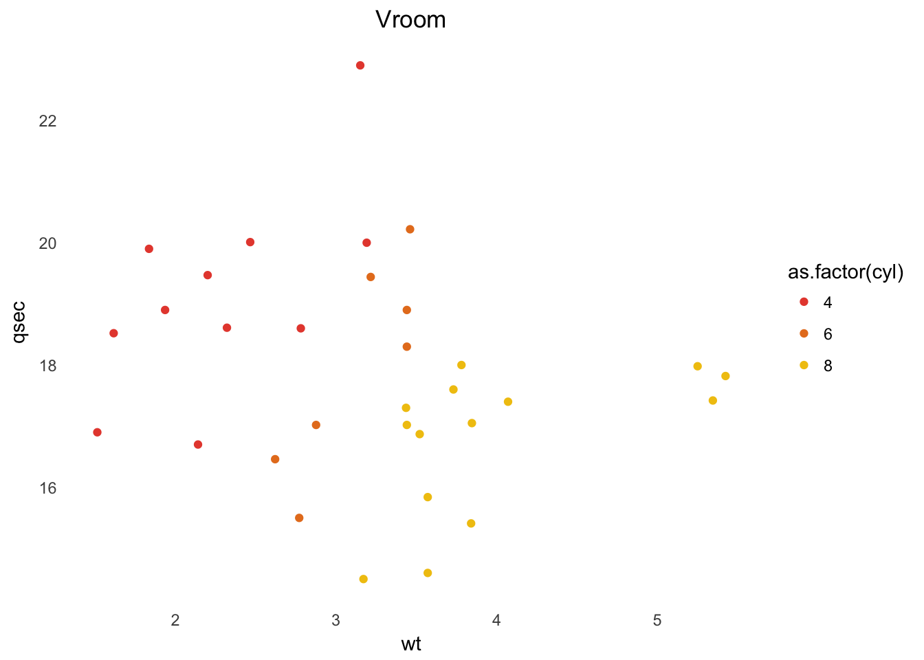

Palettes

A number of palettes are available through the pal() function. A visual overview can be acquired as follows:

plot_palettes()

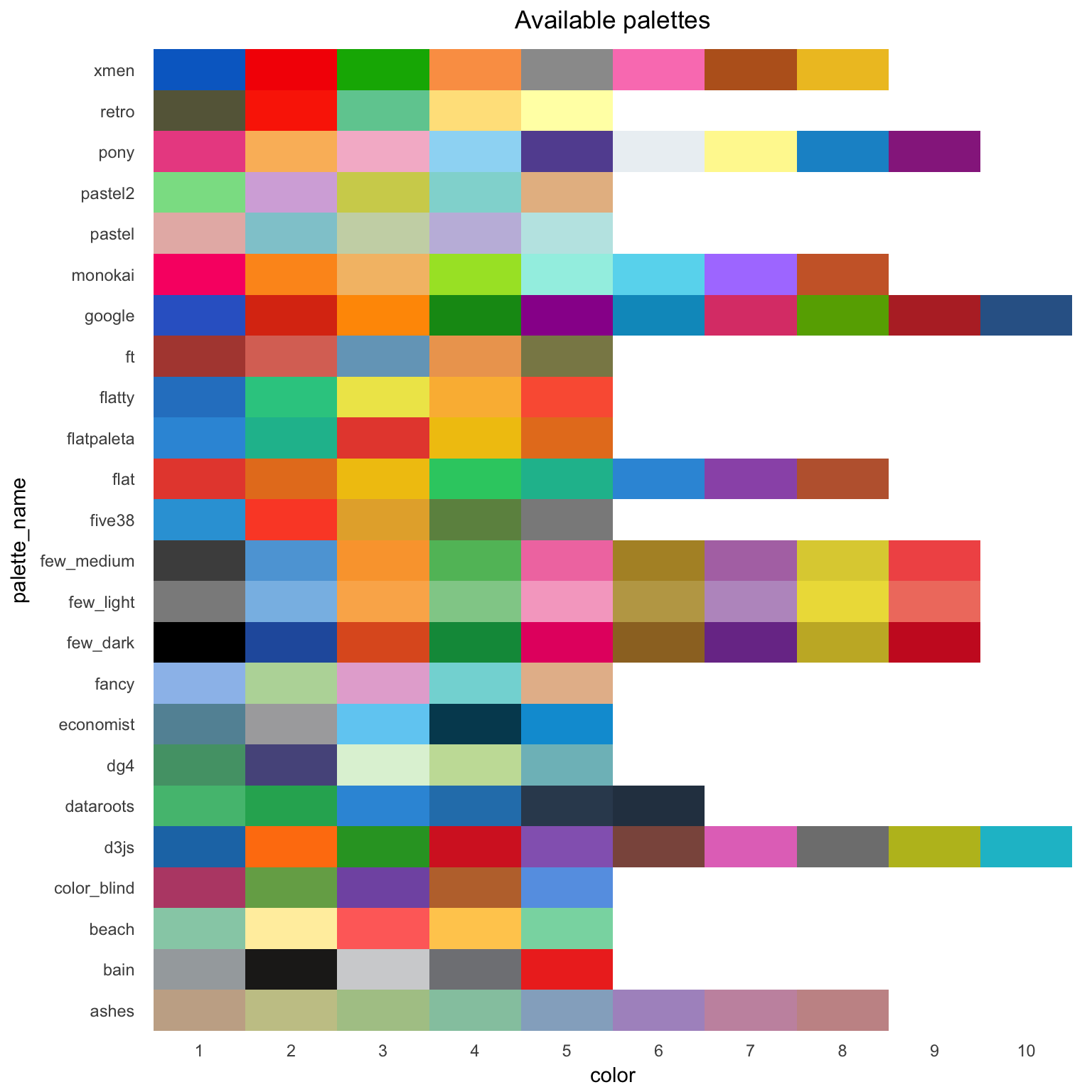
Check out the examples above to see how these palettes can be applied, refer to the ?pal() documentation for more details

Watermarks

A watermark might not add much value to a plot, but there are times that you just need to be able to to add a simple watermark.

ggplot(diamonds) +
  geom_bar(aes(cut, fill=cut)) +
  theme_retro() +
  ggtitle("Sparkly stones") +
  scale_fill_manual(values = pal("retro")) +
  watermark_img("Rlogo.png", location="tl", alpha=.5)

ggplot(mtcars) +
  geom_point(aes(x=wt, y=qsec, color=as.factor(cyl))) +
  theme_ft() +
  ggtitle("Vroom") +
  scale_color_manual(values = pal("ft")) +
  watermark_txt("watermark", location="br")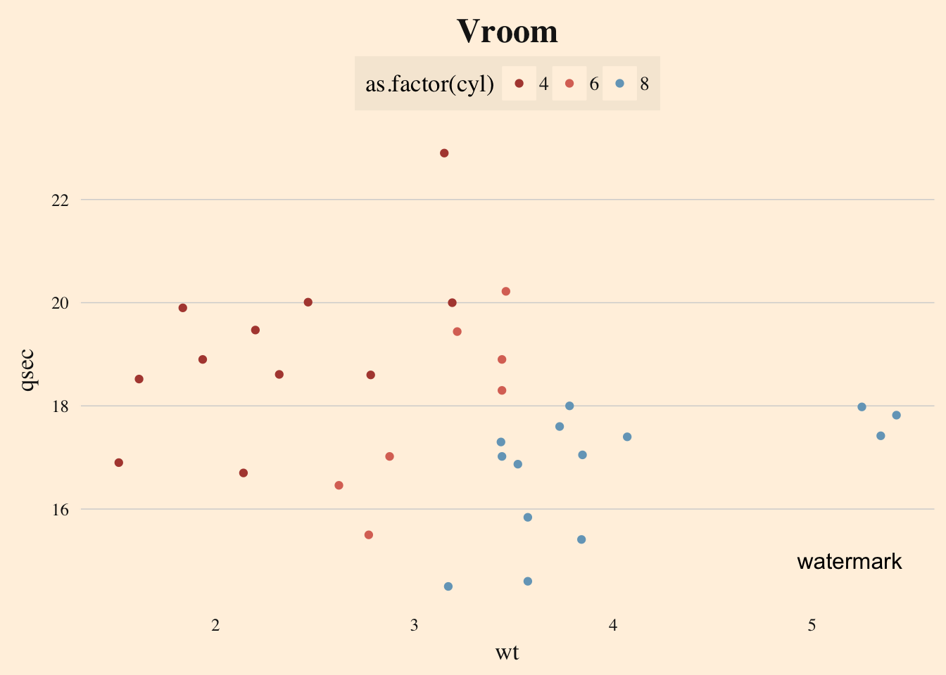

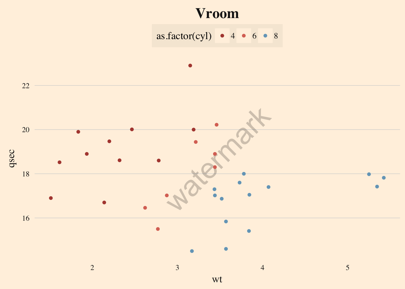
ggplot(mtcars) +
  watermark_txt("watermark", location="center", rot=45, fontsize=36, alpha=.2) +
  geom_point(aes(x=wt, y=qsec, color=as.factor(cyl))) +
  theme_ft() +
  ggtitle("Vroom") +
  scale_color_manual(values = pal("ft"))